Arkustangens und Arkuskotangens

Arkustangens und Arkuskotangens sind zwei miteinander verwandte mathematische Arkusfunktionen. Sie sind die Umkehrfunktionen der geeignet eingeschränkten Tangens- und Kotangensfunktionen: Eine Einschränkung der ursprünglichen Definitionsbereiche ist nötig, weil Tangens und Kotangens periodische Funktionen sind. Man wählt beim Tangens das Intervall ${\displaystyle ]-\pi /2,\pi /2[}$ und beim Kotangens das Intervall ${\displaystyle ]0,\pi [}$.^[1]

Zusammen mit Arkussinus und Arkuskosinus als Umkehrfunktionen des Sinus und Kosinus bildet der Arkustangens den Kern der Klasse der Arkusfunktionen. Zusammen mit den Areafunktionen sind sie in der komplexen Funktionentheorie Abwandlungen des komplexen Logarithmus, von dem sie auch die „Mehrdeutigkeit“ erben, die ihrerseits von der Periodizität der komplexen Exponentialfunktion herrührt.

Schreibweisen

Mathematische Formeln verwenden für den Arkustangens als Formelzeichen ${\displaystyle \arctan }$, ${\displaystyle \operatorname {atan} }$, ${\displaystyle \tan ^{(-1)}}$, ${\displaystyle \tan ^{\langle -1\rangle }}$ oder ${\displaystyle \tan ^{-1}}$.^[2] Für den Arkuskotangens sind die Schreibweisen ${\displaystyle \operatorname {arccot} ,}$ ${\displaystyle \operatorname {arcctg} ,}$ ${\displaystyle \operatorname {acot} }$ und neuerdings auch ${\displaystyle \cot ^{-1}}$^[3] in Gebrauch.

Aufgrund der heute für Umkehrfunktionen gebräuchlichen allgemeinen Schreibweise ${\displaystyle f^{-1}}$ beginnt dabei aber auch in diesem Fall die namentlich auf Taschenrechnern verbreitete Schreibweise ${\displaystyle \tan ^{-1}}$ die klassische Schreibweise ${\displaystyle \arctan }$ zu verdrängen, was leicht zu Verwechslungen mit dem Kehrwert des Tangens, dem Kotangens, führen kann (s. a. die Schreibweisen für die Iteration).

Eigenschaften

	Arkustangens	Arkuskotangens
Definitionsbereich	${\displaystyle x\in \mathbb {R} }$	${\displaystyle x\in \mathbb {R} }$
Bildmenge	${\displaystyle -{\tfrac {\pi }{2}}<f(x)<{\tfrac {\pi }{2}}}$	${\displaystyle 0<f(x)<\pi }$
Monotonie	streng monoton steigend	streng monoton fallend
Symmetrien	Ungerade Funktion: ${\displaystyle \arctan(-x)=-\arctan x}$	Punktsymmetrie zu ${\displaystyle \left(x=0,y={\tfrac {\pi }{2}}\right)}$ ${\displaystyle \operatorname {arccot} x=\pi -\operatorname {arccot}(-x)}$
Asymptoten	${\displaystyle f(x)\to \pm {\tfrac {\pi }{2}}}$ für ${\displaystyle x\to \pm \infty }$	${\displaystyle f(x)\to \pi }$ für ${\displaystyle x\to -\infty }$ ${\displaystyle f(x)\to 0}$ für ${\displaystyle x\to +\infty }$
Nullstellen	${\displaystyle x=0}$	keine
Sprungstellen	keine	keine
Polstellen	keine	keine
Extrema	keine	keine
Wendepunkte	${\displaystyle (0,0)}$	${\displaystyle \left(0,{\tfrac {\pi }{2}}\right)}$

Wichtige Funktionswerte

Die folgende Tabelle listet die wichtigen Funktionswerte der beiden Arkusfunktionen auf.^[4]

${\displaystyle x}$	${\displaystyle \arctan(x)}$		${\displaystyle \operatorname {arccot}(x)}$
${\displaystyle 0}$	${\displaystyle 0^{\circ }}$	${\displaystyle 0}$	${\displaystyle 90^{\circ }}$	${\displaystyle {\frac {\pi }{2}}}$
${\displaystyle {\tfrac {1}{3}}{\sqrt {3}}}$	${\displaystyle 30^{\circ }}$	${\displaystyle {\frac {\pi }{6}}}$	${\displaystyle 60^{\circ }}$	${\displaystyle {\frac {\pi }{3}}}$
${\displaystyle 1\,}$	${\displaystyle 45^{\circ }}$	${\displaystyle {\frac {\pi }{4}}}$	${\displaystyle 45^{\circ }}$	${\displaystyle {\frac {\pi }{4}}}$
${\displaystyle {\sqrt {3}}}$	${\displaystyle 60^{\circ }}$	${\displaystyle {\frac {\pi }{3}}}$	${\displaystyle 30^{\circ }}$	${\displaystyle {\frac {\pi }{6}}}$

Weitere wichtige Werte sind:

${\displaystyle x}$	${\displaystyle \arctan(x)}$		${\displaystyle \operatorname {arccot}(x)}$
${\displaystyle 2-{\sqrt {3}}}$	${\displaystyle 15^{\circ }}$	${\displaystyle {\tfrac {\pi }{12}}}$	${\displaystyle 75^{\circ }}$	${\displaystyle {\tfrac {5\pi }{12}}}$
${\displaystyle {\tfrac {1}{5}}{\sqrt {25-10{\sqrt {5}}}}}$	${\displaystyle 18^{\circ }}$	${\displaystyle {\tfrac {\pi }{10}}}$	${\displaystyle 72^{\circ }}$	${\displaystyle {\tfrac {2\pi }{5}}}$
${\displaystyle {\sqrt {5-2{\sqrt {5}}}}}$	${\displaystyle 36^{\circ }}$	${\displaystyle {\tfrac {\pi }{5}}}$	${\displaystyle 54^{\circ }}$	${\displaystyle {\tfrac {3\pi }{10}}}$
${\displaystyle {\tfrac {1}{5}}{\sqrt {25+10{\sqrt {5}}}}}$	${\displaystyle 54^{\circ }}$	${\displaystyle {\tfrac {3\pi }{10}}}$	${\displaystyle 36^{\circ }}$	${\displaystyle {\tfrac {\pi }{5}}}$
${\displaystyle {\sqrt {5+2{\sqrt {5}}}}}$	${\displaystyle 72^{\circ }}$	${\displaystyle {\tfrac {2\pi }{5}}}$	${\displaystyle 18^{\circ }}$	${\displaystyle {\tfrac {\pi }{10}}}$
${\displaystyle 2+{\sqrt {3}}}$	${\displaystyle 75^{\circ }}$	${\displaystyle {\tfrac {5\pi }{12}}}$	${\displaystyle 15^{\circ }}$	${\displaystyle {\tfrac {\pi }{12}}}$

Für Tangenswerte ${\displaystyle x>1}$ siehe die Formel im Abschnitt #Funktionalgleichungen.

Näherungsweise Berechnung

Es gelten folgende Näherungen:

Arkustangens, maximale Abweichung unter 0,005 Radianten:^[5]

${\displaystyle \arctan x\approx {\begin{cases}{\frac {x}{1+0{,}28x^{2}}}&\;\mathrm {f{\ddot {u}}r} \;|x|\leq 1\\{\frac {\pi }{2}}-{\frac {x}{x^{2}+0{,}28}}&\;\mathrm {f{\ddot {u}}r} \;x>1\\-{\frac {\pi }{2}}-{\frac {x}{x^{2}+0{,}28}}&\;\mathrm {f{\ddot {u}}r} \;x<-1\end{cases}}}$

Eine weitere Berechnungsmöglichkeit bietet CORDIC.

Arkuskotangens:

${\displaystyle \operatorname {arccot} x\approx {\frac {3x}{3x^{2}-1}}\quad \;\mathrm {f{\ddot {u}}r} \;x\gg 1}$

Reihenentwicklungen

MacLaurinsche Reihen

Die Taylorreihe des Arkustangens mit dem Entwicklungspunkt ${\displaystyle x=0}$ lautet:

${\displaystyle \arctan x=\sum _{k=0}^{\infty }(-1)^{k}{\frac {x^{2k+1}}{2k+1}}=x-{\frac {1}{3}}x^{3}+{\frac {1}{5}}x^{5}-{\frac {1}{7}}x^{7}+\dotsb }$

Die Taylorreihe des Arkuskotangens mit dem Entwicklungspunkt ${\displaystyle x=0}$ lautet:

${\displaystyle \operatorname {arccot} x={\frac {\pi }{2}}-\sum _{k=0}^{\infty }(-1)^{k}{\frac {x^{2k+1}}{2k+1}}={\frac {\pi }{2}}-x+{\frac {1}{3}}x^{3}-{\frac {1}{5}}x^{5}+{\frac {1}{7}}x^{7}-\dotsb }$

Diese Reihen konvergieren genau dann, wenn ${\displaystyle |x|\leq 1}$ und ${\displaystyle x\neq \pm \mathrm {i} }$ ist. Zur Berechnung des Arkustangens für ${\displaystyle |x|>1}$ kann man ihn auf einen Arkustangens von Argumenten mit ${\displaystyle |x|<1}$ zurückführen. Dazu kann man entweder die Funktionalgleichung benutzen oder (um ohne ${\displaystyle \pi }$ auszukommen) die Gleichung

${\displaystyle \arctan x=2\,\arctan {\frac {x}{1+{\sqrt {1+x^{2}}}}}.}$

Durch mehrfache Anwendung dieser Formel lässt sich der Betrag des Arguments beliebig verkleinern, was eine sehr effiziente Berechnung durch die Reihe ermöglicht. Schon nach einmaliger Anwendung obiger Formel hat man ein Argument mit ${\displaystyle |x|<1,}$ sodass obige Taylorreihe konvergiert, und mit jeder weiteren Anwendung wird ${\displaystyle |x|}$ mindestens halbiert, was die Konvergenzgeschwindigkeit der Taylorreihe mit jeder Anwendung der Formel erhöht.

Wegen ${\displaystyle \textstyle \cot \alpha ={\frac {1}{\tan \alpha }}}$ hat der Arkuskotangens am Entwicklungspunkt ${\displaystyle x=\infty }$ die Taylorreihe:

${\displaystyle \operatorname {arccot} x=\sum _{k=0}^{\infty }(-1)^{k}\cdot {\frac {x^{-2k-1}}{2k+1}}={\frac {1}{x}}-{\frac {1}{3x^{3}}}+{\frac {1}{5x^{5}}}-{\frac {1}{7x^{7}}}+\dotsb }$

Sie konvergiert für ${\displaystyle x\geq 1}$ und stimmt dort mit dem oben angegebenen Hauptwert überein. Sie konvergiert auch für ${\displaystyle x\leq -1,}$ allerdings mit dem Wert ${\displaystyle \operatorname {arccot} x-\pi .}$ Manche Pakete der Computeralgebra geben für ${\displaystyle x<0}$ den am Ursprung unstetigen, aber punktsymmetrischen und am unendlich fernen Punkt stetigen Wert ${\displaystyle \operatorname {arccot} x-\pi }$ als Hauptwert.

Reihen mit den Zentralbinomialkoeffizienten

Die folgenden Reihen mit den Zentralbinomialkoeffizienten konvergieren für alle Zahlen ${\displaystyle x\in \mathbb {R} }$ schnell und sind wurzelfrei:^[6]

${\displaystyle \arctan(x)=\sum _{n=1}^{\infty }{\frac {(2\,x)^{2n-1}}{n\operatorname {CBC} (n)(x^{2}+1)^{n}}}}$

${\displaystyle \arctan(x)^{2}=\sum _{n=1}^{\infty }{\frac {(2\,x)^{2n}}{2\,n^{2}\operatorname {CBC} (n)(x^{2}+1)^{n}}}}$

Der ${\displaystyle n}$-te Zentralbinomialkoeffizient für eine natürliche Zahl ${\displaystyle n}$ ist gegeben durch:

${\displaystyle \operatorname {CBC} (n)={2n \choose n}={\frac {(2n)!}{(n!)^{2}}}={\frac {\Pi (2n)}{\Pi (n)^{2}}}}$,

dabei ist   ${\displaystyle \Pi (x)=x!=\Gamma (x+1)}$   die Gaußsche Pifunktion.

Funktionalgleichungen

Statt aus Argumenten ${\displaystyle x}$ über 1 oder unter −1 lässt sich der Arkustangens aus Argumenten ${\displaystyle y={\frac {1}{x}}}$ zwischen −1 und 1 ableiten:

${\displaystyle \arctan x=\operatorname {sgn}(x)\cdot {\frac {\pi }{2}}-\arctan {\frac {1}{x}}}$.

Gleiches gilt für den Arkuskotangens:

${\displaystyle \operatorname {arccot} x=\left(2-\operatorname {sgn}(x)\right)\cdot {\frac {\pi }{2}}-\operatorname {arccot} {\frac {1}{x}}}$.

Wenn man (bspw. durch die erste Ersetzung) bei einem Argument (einem Tangenswert) ${\displaystyle y\in [0,1]}$ ankommt, kann man anschließend im Fall ${\displaystyle \textstyle y\in \left[{\frac {\sqrt {3}}{3}},1\right]}$ die Gleichung

${\displaystyle \arctan y={\frac {\pi }{4}}-{\frac {1}{2}}\cdot \arctan \left({\frac {1-y^{2}}{2y}}\right),}$

anwenden, sodass mit ${\displaystyle \textstyle z={\frac {1-y^{2}}{2y}}}$ das Argument des Arkustangens in jedem Fall (jetzt ${\displaystyle z}$, sonst ${\displaystyle y}$) ins Intervall ${\displaystyle \textstyle \left[0,{\frac {\sqrt {3}}{3}}\right]}$ mit ${\displaystyle {\tfrac {\sqrt {3}}{3}}\approx 0{,}577350\dotso }$ zu liegen kommt.

Weitere Beziehungen

${\displaystyle \operatorname {arccot} {x}={\begin{cases}\arctan \displaystyle {\frac {1}{x}}&\;\mathrm {f{\ddot {u}}r} \;x>0\\\arctan \displaystyle \left({\frac {1}{x}}\right)+\pi &\;\mathrm {f{\ddot {u}}r} \;x<0\\\end{cases}}}$

${\displaystyle \arctan {x}={\begin{cases}\operatorname {arccot} \displaystyle {\frac {1}{x}}&\;\mathrm {f{\ddot {u}}r} \;x>0\\\operatorname {arccot} \displaystyle \left({\frac {1}{x}}\right)-\pi &\;\mathrm {f{\ddot {u}}r} \;x<0\\\end{cases}}}$

${\displaystyle \operatorname {arccot} {\frac {1}{x}}-\arctan {x}=\operatorname {arccot} {x}-\arctan {\frac {1}{x}}={\begin{cases}0&\;\mathrm {f{\ddot {u}}r} \;x>0\\\pi &\;\mathrm {f{\ddot {u}}r} \;x<0\\\end{cases}}}$

${\displaystyle \arctan {x}+\operatorname {arccot} {x}={\frac {\pi }{2}}}$

Wegen der Punktsymmetrie ${\displaystyle \arctan(-x)=-\arctan(x)}$ ist mit ${\displaystyle (x,y)}$ auch ${\displaystyle (-x,-y)}$ ein Wertepaar der Arkustangensfunktion.

Additionstheoreme

Die Additionstheoreme für Arkustangens und Arkuskotangens erhält man mit Hilfe der Additionstheoreme für Tangens und Kotangens:

${\displaystyle \arctan x+\arctan y=\left\{{\begin{matrix}\arctan(\tan(\arctan x+\arctan y))=\arctan \left({\frac {x+y}{1-xy}}\right)&{\text{wenn }}xy<1\\\pi +\arctan(\tan(\arctan x+\arctan y))=\pi +\arctan \left({\frac {x+y}{1-xy}}\right)&{\text{wenn }}x+y\geq 0{\text{ und }}xy>1\\-\pi +\arctan(\tan(\arctan x+\arctan y))=-\pi +\arctan \left({\frac {x+y}{1-xy}}\right)&{\text{wenn }}x+y<0{\text{ und }}xy>1\\\end{matrix}}\right.}$

${\displaystyle \operatorname {arccot} x+\operatorname {arccot} y=\left\{{\begin{matrix}\operatorname {arccot}(\cot(\operatorname {arccot} x+\operatorname {arccot} y))=\operatorname {arccot} \left({\frac {xy-1}{x+y}}\right)&{\text{wenn }}x+y>0\\\pi +\operatorname {arccot}(\cot(\operatorname {arccot} x+\operatorname {arccot} y))=\pi +\operatorname {arccot} \left({\frac {xy-1}{x+y}}\right)&{\text{wenn }}x+y<0\\\end{matrix}}\right.}$

Daraus folgt insbesondere für doppelte Funktionswerte

${\displaystyle 2\arctan x=\left\{{\begin{matrix}\arctan \left({\frac {2x}{1-x^{2}}}\right)&{\text{wenn }}x^{2}<1\\\pi +\arctan \left({\frac {2x}{1-x^{2}}}\right)&{\text{wenn }}x\geq 0{\text{ und }}x^{2}>1\\-\pi +\arctan \left({\frac {2x}{1-x^{2}}}\right)&{\text{wenn }}x<0{\text{ und }}x^{2}>1\\\end{matrix}}\right.}$

${\displaystyle 2\operatorname {arccot} x=\left\{{\begin{matrix}\operatorname {arccot} \left({\frac {x^{2}-1}{2x}}\right)&{\text{wenn }}x>0\\\pi +\operatorname {arccot} \left({\frac {x^{2}-1}{2x}}\right)&{\text{wenn }}x<0\\\end{matrix}}\right.}$

Aus dem ersten Gesetz lässt sich für hinreichend kleine ${\displaystyle x,y}$ mit

${\displaystyle x\oplus y:=\tan(\arctan x+\arctan y)={\frac {x+y}{1-xy}}}$

das Gruppengesetz ${\displaystyle \oplus }$ ableiten. Es gilt also beispielsweise:

${\displaystyle {\frac {1}{2}}\oplus {\frac {1}{3}}={\frac {{\frac {1}{2}}+{\frac {1}{3}}}{1-{\frac {1}{6}}}}=1,}$

woraus sich

${\displaystyle \arctan {\frac {1}{2}}+\arctan {\frac {1}{3}}=\arctan {\frac {{\frac {1}{2}}+{\frac {1}{3}}}{1-{\frac {1}{6}}}}=\arctan {1}={\frac {\pi }{4}}}$

errechnet. Ferner gilt

${\displaystyle {\frac {1}{n}}\oplus {\frac {1}{4n^{3}+3n}}={\frac {4n^{3}+4n}{4n^{4}+3n^{2}-1}}={\frac {4n(n^{2}+1)}{(4n^{2}-1)(n^{2}+1)}}={\frac {4n}{4n^{2}-1}}=2\odot {\frac {1}{2n}}}$

und dementsprechend

${\displaystyle \arctan {\frac {1}{n}}=2\,\arctan {\frac {1}{2n}}-\arctan {\frac {1}{4n^{3}+3n}}.}$

Die zwei Gleichungen als Arkuskotangens geschrieben:

${\displaystyle \operatorname {arccot} {2}+\operatorname {arccot} {3}=\operatorname {arccot} {\frac {6-1}{2+3}}=\operatorname {arccot} {1}={\frac {\pi }{4}}}$

und

${\displaystyle \operatorname {arccot} {n}=2\,\operatorname {arccot}(2n)-\operatorname {arccot}(4n^{3}+3n).}$

Berechnung der Kreiszahl π mit Hilfe des Arkustangens

Die Reihenentwicklung kann dazu verwendet werden, die Zahl π mit beliebiger Genauigkeit zu berechnen: Die einfachste Formel ist der Spezialfall ${\displaystyle x=1,}$ die Leibniz-Formel

${\displaystyle {\frac {\pi }{4}}=1-{\frac {1}{3}}+{\frac {1}{5}}-{\frac {1}{7}}+\dotsb }$

Da sie nur extrem langsam (logarithmisch) konvergiert, verwendete John Machin 1706 die Formel

${\displaystyle {\frac {\pi }{4}}=4\,\operatorname {arccot} {5}-\operatorname {arccot} {239},}$

um die ersten 100 Nachkommastellen von ${\displaystyle \pi }$ mit Hilfe der Taylorreihe für den Arkustangens zu berechnen. Letztere konvergiert schneller (linear) und wird auch heute noch für die Berechnung von ${\displaystyle \pi }$ verwendet.

Im Laufe der Zeit wurden noch mehr Formeln dieser Art gefunden. Ein Beispiel stammt von Carl Størmer (1896):

${\displaystyle {\frac {\pi }{4}}=44\,\operatorname {arccot} {57}+7\,\operatorname {arccot} {239}-12\,\operatorname {arccot} {682}+24\,\operatorname {arccot} {12943},}$^[7]

was gleichbedeutend damit ist, dass der Realteil und der Imaginärteil der Gaußschen Zahl

${\displaystyle (57+\mathrm {i} )^{44}\,(239+\mathrm {i} )^{7}\,(682-\mathrm {i} )^{12}\,(12943+\mathrm {i} )^{24}=(1+\mathrm {i} )\cdot n}$ mit ${\displaystyle n\in \mathbb {Z} }$

gleich sind.^[8]

Gleiches gilt für die Formel von John Machin, wobei es hier um die Gaußsche Zahl

${\displaystyle (5+\mathrm {i} )^{4}\,(239-\mathrm {i} )=(1+\mathrm {i} )\cdot 114244}$

geht, die mit einem Taschenrechner berechnet werden kann.

Komplexer Arkustangens und Arkuskotangens

Lässt man komplexe Argumente und Werte zu, so hat man

${\displaystyle \arctan(a+b\,\mathrm {i} )=\left\{{\begin{array}{ll}\displaystyle {\frac {1}{2}}\,\left(\arctan {\frac {a^{2}+b^{2}-1}{2a}}+{\frac {\pi }{2}}\,\operatorname {sgn}(a)\right)&\;a\neq 0\\0&\;a=0,\,|b|\leq 1\\\displaystyle {\frac {\pi }{2}}\,\operatorname {sgn}(b)&\;a=0,\,|b|>1\\\end{array}}\right\}}$ ${\displaystyle {}+\mathrm {i} \cdot {\frac {1}{2}}\,\operatorname {artanh} {\frac {2b}{a^{2}+b^{2}+1}}}$  mit ${\displaystyle a,b\in \mathbb {R} ,}$

eine Darstellung, die quasi schon in Real- und Imaginärteil aufgespalten ist. Wie im Reellen gilt

${\displaystyle \operatorname {arccot}(z)={\frac {\pi }{2}}-\arctan(z)}$

mit ${\displaystyle z=a+b\,\mathrm {i} .}$

Man kann im Komplexen sowohl den Arkustangens (wie auch den Arkuskotangens) durch ein Integral und durch den komplexen Logarithmus ausdrücken:

${\displaystyle {\begin{array}{ll}\displaystyle \arctan z=\int _{0}^{z}{\frac {\mathrm {d} t}{1+t^{2}}}&\displaystyle ={\frac {1}{2}}\,\int _{0}^{z}\left({\frac {\mathrm {d} t}{1+\mathrm {i} t}}+{\frac {\mathrm {d} t}{1-\mathrm {i} t}}\right)\\\displaystyle ={\frac {\ln(1+\mathrm {i} z)-\ln(1-\mathrm {i} z)}{2\mathrm {i} }}&\displaystyle ={\frac {1}{2\mathrm {i} }}\,\ln {\frac {1+\mathrm {i} z}{1-\mathrm {i} z}}\end{array}}}$

für ${\displaystyle z}$ in der zweifach geschlitzten Ebene ${\displaystyle {}^{|}\mathbb {C} _{|}:=\mathbb {C} \setminus \{\mathrm {i} y\,|\,y\in \mathbb {R} ,|y|\geq 1\}.}$ Das Integral hat einen Integrationsweg, der die imaginäre Achse nicht kreuzt außer evtl. im Einheitskreis. Es ist in diesem Gebiet ${\displaystyle {}^{|}\mathbb {C} _{|}}$ regulär und eindeutig.^[9]

Der Arkustangens spielt eine wesentliche Rolle bei der symbolischen Integration von Ausdrücken der Form

${\displaystyle {\frac {1}{ax^{2}+bx+c}}.}$

Ist die Diskriminante ${\displaystyle D=b^{2}-4ac}$ nichtnegativ, so kann man eine Stammfunktion mittels Partialbruchzerlegung bestimmen. Ist die Diskriminante negativ, so kann man den Ausdruck durch die Substitution

${\displaystyle t={\frac {2ax+b}{\sqrt {-D}}}}$

in die Form

${\displaystyle {\frac {4a}{-D}}\,{\frac {1}{1+t^{2}}}}$

bringen; eine Stammfunktion ist also

${\displaystyle {\frac {2}{\sqrt {-D}}}\,\arctan {\frac {2ax+b}{\sqrt {-D}}}.}$

Und so entsteht das Endresultat:

${\displaystyle {\frac {1}{ax^{2}+bx+c}}={\frac {\mathrm {d} }{\mathrm {d} x}}{\biggl [}{\frac {2}{\sqrt {4ac-b^{2}}}}\arctan {\biggl (}{\frac {2ax+b}{\sqrt {4ac-b^{2}}}}{\biggr )}{\biggr ]}}$

Umrechnung ebener kartesischer Koordinaten in polare

Ist ein Punkt ${\displaystyle {\mathsf {P}}}$ in der Ebene durch Polarkoordinaten ${\displaystyle (r,\varphi )}$ gegeben, so sind seine kartesischen Koordinaten ${\displaystyle (x,y)}$ durch die Gleichungen

${\displaystyle {\begin{array}{ll}x=r\cdot \cos(\varphi )\\y=r\cdot \sin(\varphi )\\\end{array}}}$

${\displaystyle {\biggr \}}\;({\text{P}}\to {\text{K}})}$

bestimmt.

Die Umrechnung in der Gegenrichtung ist etwas komplizierter. Auf jeden Fall gehört der Abstand

${\displaystyle r={\sqrt {x^{2}+y^{2}}}}$

${\displaystyle ({\text{K}}\to {\text{P}}_{r})}$

des Punktes ${\displaystyle {\mathsf {P}}}$ vom Ursprung ${\displaystyle {\mathsf {O}}(0,0)}$ zur Lösung. Ist nun ${\displaystyle r=0,}$ dann ist auch ${\displaystyle x=y=0,}$ und es spielt keine Rolle, welchen Wert ${\displaystyle \varphi \in \mathbb {R} }$ hat. Dieser Fall wird im Folgenden als der singuläre Fall bezeichnet.

Ist aber ${\displaystyle r\neq 0,}$ dann ist ${\displaystyle \varphi ,}$ weil die Funktionen ${\displaystyle \sin }$ und ${\displaystyle \cos }$ die Periode ${\displaystyle 2\pi }$ haben, durch die Gleichungen ${\displaystyle ({\text{P}}\to {\text{K}})}$ nur modulo ${\displaystyle 2\pi \mathbb {Z} }$ bestimmt, d. h., mit ${\displaystyle \varphi }$ ist auch ${\displaystyle \varphi +2\pi n}$ für jedes ${\displaystyle n\in \mathbb {Z} }$ eine Lösung.

Trigonometrische Umkehrfunktionen sind erforderlich, um von Längen zu Winkeln zu kommen. Hier zwei Beispiele, bei denen der Arkustangens zum Einsatz kommt.

Der simple Arkustangens ${\displaystyle \varphi =\arctan \left({\frac {y}{x}}\right)}$ (s. Abb. 3) reicht allerdings nicht aus. Denn wegen der Periodizität des Tangens von ${\displaystyle \pi }$ muss dessen Definitionsmenge vor der Umkehrung auf eine Periodenlänge von ${\displaystyle \pi }$ eingeschränkt werden, was zur Folge hat, dass die Umkehrfunktion (der Arkustangens) keine größere Bildmenge haben kann.

Halber Winkel

In der nebenstehenden Abb. 3^[10] ist die Polarachse (die mit der ${\displaystyle +x}$-Achse definitionsgemäß zusammenfällt) um den Betrag ${\displaystyle r}$ in die ${\displaystyle -x}$-Richtung verlängert, also vom Pol (und Ursprung) ${\displaystyle {\mathsf {O}}}$ bis zum Punkt ${\displaystyle {\mathsf {N}}.}$ Das Dreieck ${\displaystyle {\mathsf {NOP}}}$ ist ein gleichschenkliges, sodass die Winkel ${\displaystyle \sphericalangle {\mathsf {PNO}}}$ und ${\displaystyle \sphericalangle {\mathsf {OPN}}}$ gleich sind. Ihre Summe, also das Doppelte eines von ihnen, ist gleich dem Außenwinkel ${\displaystyle \varphi }$ des Dreiecks ${\displaystyle {\mathsf {NOP}}.}$ Dieser Winkel ist der gesuchte Polarwinkel ${\displaystyle \sphericalangle {\mathsf {XOP}}.}$ Mit dem Abszissenpunkt ${\displaystyle {\mathsf {A}}}$ gilt im rechtwinkligen Dreieck ${\displaystyle {\mathsf {NAP}}}$

${\displaystyle \tan \left({\frac {\varphi }{2}}\right)={\frac {|{\text{Gegenkathete }}{\mathsf {PA}}|}{|{\text{Ankathete }}{\mathsf {AN}}|}}={\frac {y}{r+x}},}$

was nach ${\displaystyle \varphi }$ aufgelöst

${\displaystyle \varphi =2\cdot \arctan \left({\frac {y}{r+x}}\right)}$

${\displaystyle ({\text{K}}\to {\text{P}}_{\varphi }(A))}$

ergibt. Die Gleichung versagt, wenn ${\displaystyle r+x=0}$ ist. Dann muss wegen ${\displaystyle |x|\leq |r|\Rightarrow x=-|r|}$ auch ${\displaystyle y=0}$ sein. Wenn jetzt ${\displaystyle x=0}$ ist, dann handelt es sich um den singulären Fall. Ist aber ${\displaystyle x<0,}$ dann sind die Gleichungen ${\displaystyle ({\text{P}}\to {\text{K}})}$ durch ${\displaystyle \varphi =+\pi }$ oder ${\displaystyle \varphi =-\pi }$ erfüllt.^[11] Das ist in Einklang mit den Bildmengen ${\displaystyle ]-\pi ,+\pi ]}$ resp. ${\displaystyle [-\pi ,+\pi [}$ der Funktion im folgenden Abschnitt.

Der „Arkustangens“ mit zwei Argumenten

Ein anderer Weg, um zu einem vollwertigen Polarwinkel zu kommen, ist in vielen Programmiersprachen und Tabellenkalkulationen gewählt worden, und zwar eine erweiterte Funktion, die mit den beiden kartesischen Koordinaten beschickt wird und die damit genügend Information hat, um den Polarwinkel modulo ${\displaystyle 2\pi \mathbb {Z} ,}$ bspw. im Intervall ${\displaystyle ]-\pi ,\pi ],}$ und in allen vier Quadranten zurückgeben zu können:

${\displaystyle \varphi =\operatorname {arctan2} (x,y)}$

${\displaystyle ({\text{K}}\to {\text{P}}_{\varphi }(B))}$

Zusammen mit der Gleichung ${\displaystyle {\color {Blue}({\text{K}}\to {\text{P}}_{r})}}$ erfüllt jede der beiden Lösungen ${\displaystyle {\color {Blue}({\text{K}}\to {\text{P}}_{\varphi }(A))}}$ und ${\displaystyle {\color {Blue}({\text{K}}\to {\text{P}}_{\varphi }(B))}}$ die Gleichungen ${\displaystyle {\color {Blue}({\text{P}}\to {\text{K}})}}$:

${\displaystyle x=r\cos \varphi }$       und

${\displaystyle y=r\sin \varphi }$ ,

und zwar für ${\displaystyle (x,y)=(0,0)}$ mit jedem beliebigen ${\displaystyle \varphi \in \mathbb {R} .}$

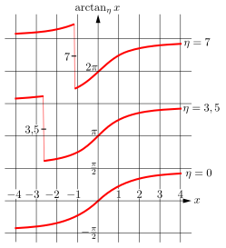
Arkustangens mit Lageparameter

In vielen Anwendungsfällen soll die Lösung ${\displaystyle y}$ der Gleichung ${\displaystyle x=\tan y}$ so nahe wie möglich bei einem gegebenen Wert ${\displaystyle \eta }$ liegen. Dazu eignet sich die mit dem Parameter ${\displaystyle \eta }$ modifizierte Arkustangens-Funktion

${\displaystyle y=\arctan _{\eta }x:=\arctan x+\pi \cdot \operatorname {rni} {\frac {\eta -\arctan x}{\pi }}.}$

Die Funktion ${\displaystyle \operatorname {rni} }$ rundet zur engstbenachbarten ganzen Zahl.

Ableitungen

Arkustangens:

${\displaystyle {\frac {\mathrm {d} }{\mathrm {d} x}}\arctan(x)={\frac {1}{1+x^{2}}}}$

Arkuskotangens:

${\displaystyle {\frac {\mathrm {d} }{\mathrm {d} x}}\operatorname {arccot}(x)=-{\frac {1}{1+x^{2}}}}$

Integrale

Standardisierte Integraldarstellungen

Arkustangens und Arkuskotangens haben folgende standardisierte Integraldarstellungen:

${\displaystyle \arctan(x)=\int _{0}^{x}{\frac {1}{t^{2}+1}}\,\mathrm {d} t=\int _{0}^{1}{\frac {x}{x^{2}y^{2}+1}}\,\mathrm {d} y}$

${\displaystyle \operatorname {arccot}(x)=\int _{x}^{\infty }{\frac {1}{t^{2}+1}}\,\mathrm {d} t={\frac {\pi }{2}}-\int _{0}^{1}{\frac {x}{x^{2}y^{2}+1}}\,\mathrm {d} y}$

Arkustangens und Gaußsches Fehlerintegral

Die Arkustangensfunktion hat folgende Integralidentität mit der Gaussschen Fehlerfunktion erf(x):

${\displaystyle \arctan(x)=\int _{0}^{\infty }{\sqrt {\pi }}\,\exp(-y^{2})\,\mathrm {erf} (xy)\,\mathrm {d} y}$

Mit der nicht normierten Fehlerfunktion kann diese Identität auch so geschrieben werden:

${\displaystyle \arctan(x)=\int _{0}^{\infty }2\exp(-y^{2})\,\mathrm {erf} ^{*}(xy)\,\mathrm {d} y}$

${\displaystyle \mathrm {erf} ^{*}(v)=\int _{0}^{v}\exp(-w^{2})\,\mathrm {d} w}$

Durch Ableiten dieser Integralidentität entsteht die Ableitung des Arkustangens:

${\displaystyle {\frac {\mathrm {d} }{\mathrm {d} x}}\int _{0}^{\infty }2\exp(-y^{2})\,\mathrm {erf} ^{*}(xy)\,\mathrm {d} y=\int _{0}^{\infty }2y\exp(-y^{2})\exp(-x^{2}y^{2})\,\mathrm {d} y=}$

${\displaystyle =\int _{0}^{\infty }2y\exp {\bigl [}-(x^{2}+1)\,y^{2}{\bigr ]}\,\mathrm {d} y={\frac {1}{x^{2}+1}}}$

Die genannte Integralidentität ist bezüglich x eine Ursprungsfunktion.

Wenn der Wert ${\displaystyle x=1}$ eingesetzt wird, dann wird folgender Zusammenhang sichtbar:

${\displaystyle {\frac {\pi }{4}}=\arctan(1)=\int _{0}^{\infty }2\exp(-y^{2})\,\mathrm {erf} ^{*}(y)\,\mathrm {d} y={\biggl [}\,\mathrm {erf} ^{*}(y)^{2}{\biggr ]}_{y=0}^{y=\infty }=\lim _{y\rightarrow \infty }\mathrm {erf} ^{*}(y)^{2}}$

${\displaystyle \int _{0}^{\infty }\exp(-x^{2})\,\mathrm {d} x=\lim _{y\rightarrow \infty }\mathrm {erf} ^{*}(y)={\frac {1}{2}}{\sqrt {\pi }}}$

Mit der genannten Identität des Arkustangens kann somit das Integral der Gaussschen Glockenkurve bewiesen werden.

Integralidentität mit dem Logarithmus Naturalis

Auch mit dem Logarithmus Naturalis kann für den Arkustangens eine Integralidentität aufgestellt werden:

${\displaystyle \arctan(x)=\int _{0}^{1}{\frac {1}{\pi y}}\ln {\biggl [}{\frac {{\sqrt {x^{2}+1}}(y^{2}+1)+2xy}{{\sqrt {x^{2}+1}}(y^{2}+1)-2xy}}{\biggr ]}\,\mathrm {d} y}$

Durch Ableiten dieser Integralidentität entsteht ebenso die Ableitung des Arkustangens:

${\displaystyle {\frac {\mathrm {d} }{\mathrm {d} x}}\int _{0}^{1}{\frac {1}{\pi y}}\ln {\biggl [}{\frac {{\sqrt {x^{2}+1}}(y^{2}+1)+2xy}{{\sqrt {x^{2}+1}}(y^{2}+1)-2xy}}{\biggr ]}\,\mathrm {d} y=\int _{0}^{1}{\frac {4(y^{2}+1)}{\pi {\sqrt {x^{2}+1}}{\bigl [}(x^{2}+1)(y^{4}+1)+2(-x^{2}+1)\,y^{2}{\bigr ]}}}\,\mathrm {d} y={\frac {1}{x^{2}+1}}}$

Die genannte Integralidentität ist bezüglich x eine Ursprungsfunktion.

Die nun gezeigte Integralidentität wurde durch den Mathematiker James Harper entdeckt und in seinem Werk Another simple proof^[12] aus dem Jahre 2003 behandelt.

Wenn der Grenzwert von dieser Identität für ${\displaystyle x\rightarrow \infty }$ berechnet wird, dann entsteht für dieses Integral über den Areatangens Hyperbolicus folgende Identität:

${\displaystyle \int _{0}^{1}{\frac {1}{y}}\,\mathrm {artanh} (y)\,\mathrm {d} y={\frac {\pi ^{2}}{8}}}$

Und mit dieser Formel kann das Basler Problem gelöst werden.

Ebenso kann für das Quadrat des Arkustangens eine Logarithmus-Naturalis-Integralidentität aufgestellt werden:

${\displaystyle \arctan(x)^{2}=\int _{0}^{1}{\frac {1}{2z}}\ln {\biggl [}{\frac {(x^{2}+1)(z+1)^{2}}{(x^{2}+1)(z^{2}+1)+2(1-x^{2})z}}{\biggr ]}\,\mathrm {d} z}$

Ursprüngliche Stammfunktionen

Das sind die direkten Stammfunktionen der beiden behandelten Arkusfunktionen:

Arkustangens:

Die Ursprungsstammfunktion des Arkustangens lautet so:

${\displaystyle \int _{0}^{x}\arctan(y)\,\mathrm {d} y=\int _{0}^{1}x\arctan(xz)\,\mathrm {d} z=x\arctan(x)-{\frac {1}{2}}\ln(1+x^{2})}$

Nach dem Fundamentalsatz der Infinitesimalrechnung gilt somit:

${\displaystyle {\frac {\mathrm {d} }{\mathrm {d} x}}{\biggl [}x\arctan(x)-{\frac {1}{2}}\ln(1+x^{2}){\biggr ]}=\arctan(x)}$

Arkuskotangens:

Die Ursprungsstammfunktion des Arkuskotangens ist diese Funktion:

${\displaystyle \int _{0}^{x}\operatorname {arccot}(y)\,\mathrm {d} y=\int _{0}^{1}x\operatorname {arccot}(xz)\,\mathrm {d} z=x\operatorname {arccot}(x)+{\frac {1}{2}}\ln(1+x^{2})}$

Analog zum vorherigen Fall gilt damit:

${\displaystyle {\frac {\mathrm {d} }{\mathrm {d} x}}{\biggl [}x\operatorname {arccot}(x)+{\frac {1}{2}}\ln(1+x^{2}){\biggr ]}=\operatorname {arccot}(x)}$

Von einer ursprünglichen Stammfunktion auf die jeweils andere kann außerdem mit dieser Beziehung direkt gefolgert werden:

${\displaystyle \operatorname {arccot}(x)+\arctan(x)={\frac {\pi }{2}}}$

Stammfunktion des kardinalisierten Arkustangens

Der kardinalisierte Arkustangens hat das sogenannte Arkustangensintegral (Inverse Tangent Integral)^[13] als ursprüngliche Stammfunktion:

${\displaystyle \int _{0}^{x}{\frac {1}{y}}\arctan(y)\,\mathrm {d} y=\int _{0}^{1}{\frac {1}{z}}\arctan(xz)\,\mathrm {d} z=\operatorname {Ti} _{2}(x)}$

Diese Funktion zählt zu den Polylogarithmen und bildet zu der Legendresche Chifunktion ${\displaystyle \chi _{2}}$ das imaginäre Gegenstück.

Die Catalansche Konstante ist das bekannteste Beispiel für einen Wert dieser Stammfunktion:

${\displaystyle \int _{0}^{1}{\frac {1}{x}}\arctan(x)\,\mathrm {d} x=\operatorname {Ti} _{2}(1)=\beta (2)=G}$

Mit dem kleinen Beta wird hierbei die Dirichletsche Betafunktion dargestellt.

Dies sind zwei weitere Funktionswerte für das Arkustangensintegral:

${\displaystyle \operatorname {Ti} _{2}(2-{\sqrt {3}})={\tfrac {2}{3}}G-{\tfrac {1}{12}}\pi \operatorname {arcosh} (2)}$

${\displaystyle \operatorname {Ti} _{2}(2+{\sqrt {3}})={\tfrac {2}{3}}G+{\tfrac {5}{12}}\pi \operatorname {arcosh} (2)}$

Diese Bilanz stellt eine Beziehung zur Funktion Areasinus Hyperbolicus her:

${\displaystyle \operatorname {Ti} _{2}({\sqrt {x^{2}+1}}+x)-\operatorname {Ti} _{2}({\sqrt {x^{2}+1}}-x)={\tfrac {1}{2}}\pi \operatorname {arsinh} (x)}$

Zur Ursprungsstammfunktion des kardinalisierten Arkussinus, dem sogenannten Arkussinusintegral hat das Arkustangensintegral diese Identität:

${\displaystyle 2\,\mathrm {Ti} _{2}{\bigl [}x(1+{\sqrt {1-x^{2}}})^{-1}{\bigr ]}=4\,\mathrm {Si} _{2}{\bigl (}{\tfrac {1}{2}}{\sqrt {1+x}}-{\tfrac {1}{2}}{\sqrt {1-x}}\,{\bigr )}-\mathrm {Si} _{2}(x)}$

Summenreihen mit dem Arkustangens

Einige Arkustangenssummen divergieren:

${\displaystyle \sum _{n=1}^{\infty }\arctan \left({\frac {1}{n}}\right)=+\infty }$

Vergleichsformel ohne Arkustangens:

${\displaystyle \sum _{n=1}^{\infty }{\frac {1}{n}}=+\infty }$

Andere Arkustangenssummen konvergieren:

${\displaystyle \sum _{n=1}^{\infty }\arctan \left({\frac {1}{n^{2}}}\right)={\frac {\pi }{4}}+\arctan \left[-\cot \left({\frac {1}{2}}{\sqrt {2}}\,\pi \right)\tanh \left({\frac {1}{2}}{\sqrt {2}}\,\pi \right)\right]\approx 1{,}42474177842998}$

Die Abkürzung tanh bringt die Funktion Tangens Hyperbolicus zum Ausdruck.

Vergleichsformel ohne Arkustangens:

${\displaystyle \sum _{n=1}^{\infty }{\frac {1}{n^{2}}}={\frac {\pi ^{2}}{6}}\approx 1{,}644934066848}$

Folgende Formel handelt von den Fibonacci-Zahlen und ergibt ein einfaches Resultat:

${\displaystyle \sum _{n=1}^{\infty }\arctan \left({\frac {1}{f_{2n-1}}}\right)={\frac {\pi }{2}}\approx 1{,}5707963267948966}$

Denn für alle natürlichen Zahlen ${\displaystyle n}$ gilt dieser^[14] Zusammenhang:

${\displaystyle \arctan \left({\frac {1}{f_{2n}}}\right)=\arctan \left({\frac {1}{f_{2n+1}}}\right)+\arctan \left({\frac {1}{f_{2n+2}}}\right)}$

Mit der Tangenssumme ausgedrückt:

${\displaystyle {\frac {1}{f_{2n}}}={\frac {1}{f_{2n+1}}}\oplus {\frac {1}{f_{2n+2}}}}$

Dagegen ergibt die Vergleichsformel ohne Arkustangens ein elliptisches^[15][16] Resultat:

${\displaystyle \sum _{n=1}^{\infty }{\frac {1}{f_{2n-1}}}={\frac {\sqrt {5}}{8}}\left[\vartheta _{00}(\varphi )^{2}-\vartheta _{01}(\varphi )^{2}\right]\approx 1{,}8245151574}$

${\displaystyle \varphi ={\frac {1}{2}}\left({\sqrt {5}}-1\right)}$

Die kleinen griechischen Thetasymbole stellen die Jacobische Thetafunktion dar.

Die Summenreihen mit dem Arkustangens als Summanden dienen auch zur Beschreibung einiger Funktionen. Beispielsweise hat die Gudermannfunktion für alle reellen Zahlen ${\displaystyle x}$ diese Identität:

${\displaystyle \operatorname {gd} (x)=\sum _{n=1}^{\infty }\left\{2\arctan \left[{\frac {2\,x}{(4n-3)\,\pi }}\right]-2\arctan \left[{\frac {2\,x}{(4n-1)\,\pi }}\right]\right\}}$

Diese Summenreihe geht als Ursprungsstammfunktion aus der Cauchyschen Summenreihe für den Sekans Hyperbolicus hervor:

${\displaystyle \operatorname {sech} (x)=\sum _{n=1}^{\infty }\left[{\frac {(16n-12)\,\pi }{(4n-3)^{2}\,\pi ^{2}+4\,x^{2}}}-{\frac {(16n-4)\,\pi }{(4n-1)^{2}\,\pi ^{2}+4\,x^{2}}}\right]}$

Siehe auch

• Formelsammlung Trigonometrie
• Størmer-Zahl
• Trigonometrische Funktionen

Literatur

• I. N. Bronstein, K. A. Semendjajev, G. Musiol, H. Mühlig (Hrsg.): Taschenbuch der Mathematik. 7., vollständig überarbeitete und ergänzte Auflage. Verlag Harri Deutsch, Frankfurt am Main 2008, ISBN 978-3-8171-2007-9, S. 85–88. 
• G.Huvent: Autour de la primitive de tp coth (αt/2). 3. Februar 2002. Seite 5
• Mircea Ivan: A simple solution to Basel problem. General Mathematics Vol. 16, No. 4, Technical University of Cluj-Napoca Department of Mathematics, 2008
• James D. Harper: A simple proof of ${\displaystyle 1+1/2^{2}+1/3^{2}+\ldots =\pi ^{2}/6}$ The American Mathematical Monthly 109(6) (Jun. - Jul., 2003) 540–541.

Weblinks

Einzelnachweise und Anmerkungen

1. ↑ Beide Funktionen sind monoton in diesen Intervallen, und diese sind von den jeweiligen Polstellen begrenzt.
2. ↑ Eric W. Weisstein: Inverse Tangent. In: MathWorld (englisch).
3. ↑ Eric W. Weisstein: Inverse Cotangent. In: MathWorld (englisch).
4. ↑ Georg Hoever: Höhere Mathematik kompakt. Springer Spektrum, Berlin Heidelberg 2014, ISBN 978-3-662-43994-4 (eingeschränkte Vorschau in der Google-Buchsuche). 
5. ↑ Weitere Approximationen (en) (Memento vom 16. April 2009 im Internet Archive)
6. ↑ Derrick Henry Lehmer: Interesting Series Involving the Central Binomial Coefficient. Volume 92, 1985. Seite 452
7. ↑ Bspw. sind die Zahlen ${\displaystyle 1,2,4,5,\dotsc }$ Størmer-Zahlen;
   ${\displaystyle 3,\dotso ,57,\dotso ,239,\dotso ,682,\dotso ,12943,\dotso }$ dagegen nicht.
8. ↑ Dabei ist ${\displaystyle n\approx 2{,}84438\dotso \cdot 10^{226}.}$
9. ↑ Milton Abramowitz und Irene Stegun: Handbook of Mathematical Functions. (1964) Dover Publications, New York. ISBN 0-486-61272-4 Formel 4.4.3
10. ↑ Eine ganz ähnliche Skizze ist die von Einheitskreis#Rationale Parametrisierung.
11. ↑ Beim Rechnen mit Gleitkommazahlen besteht Instabilität in der Nähe des ${\displaystyle -x}$-Strahls wegen ${\displaystyle |r+x|\ll 1.}$
12. ↑ James D.Harper, Another simple proof of ${\displaystyle 1+{\frac {1}{2^{2}}}+{\frac {1}{3^{2}}}+\cdots ={\frac {\pi ^{2}}{6}}}$, American Mathematical Monthly, Band 110, Nr. 6, 2003, S. 540–541
13. ↑ Eric W. Weisstein: Inverse Tangent Integral. Abgerufen am 31. Oktober 2023 (englisch). 
14. ↑ Fibonacci numbers and the arctangent function - ProQuest. Abgerufen am 4. Dezember 2022. 
15. ↑ Eric W. Weisstein: Reciprocal Fibonacci Constant. Abgerufen am 4. Dezember 2022 (englisch). 
16. ↑ Number-theoretical, combinatorial and integer functions — mpmath 1.1.0 documentation. Abgerufen am 4. Dezember 2022.