Gauß-Quadratur

Die Gauß-Quadratur (nach Carl Friedrich Gauß) ist ein Verfahren zur numerischen Integration, das bei gegebenen Freiheitsgraden eine optimale Approximation des Integrals liefert. Bei diesem Verfahren wird die zu integrierende Funktion ${\displaystyle f}$ aufgeteilt in ${\displaystyle f(x)=w(x)\cdot \Phi (x)}$, wobei ${\displaystyle w}$ eine Gewichtsfunktion ist und ${\displaystyle \Phi }$ durch ein spezielles Polynom mit speziell gewählten Auswertungspunkten ${\displaystyle x_{i}}$ approximiert wird. Dieses Polynom lässt sich exakt integrieren. Das Verfahren ist also von der Form

${\displaystyle \int _{a}^{b}f(x)\,\mathrm {d} x=\int _{a}^{b}\Phi (x)w(x)\,\mathrm {d} x\approx \int _{a}^{b}p_{n}(x)w(x)\,\mathrm {d} x=\sum _{i=1}^{n}\Phi (x_{i})\alpha _{i}}$.

Die Gewichtsfunktion ${\displaystyle w}$ ist größer gleich Null, hat endlich viele Nullstellen und ist integrierbar. ${\displaystyle \Phi }$ ist eine stetige Funktion. Der Integrationsbereich ${\displaystyle [a,b]}$ ist nicht auf endliche Intervalle beschränkt. Weiterhin werden ${\displaystyle x_{i}}$ als Knoten, Abszissenwerte oder Stützstellen und die Größen ${\displaystyle \alpha _{i}}$ als Gewichte bezeichnet.

Das Verfahren wurde 1814 von Gauß veröffentlicht,^[1] und Carl Gustav Jacobi hat es 1826 in die heutige Form mit orthogonalen Polynomen gebracht.^[2]

Eigenschaften

Um optimale Genauigkeit zu erreichen, müssen die Abszissenwerte ${\displaystyle x_{i}}$ einer Gauß-Quadraturformel vom Grad ${\displaystyle n}$ genau den Nullstellen des ${\displaystyle n}$-ten orthogonalen Polynoms ${\displaystyle P_{n}}$ vom Grad ${\displaystyle n}$ entsprechen. Die Polynome ${\displaystyle P_{1}}$, ${\displaystyle P_{2}}$, …, ${\displaystyle P_{n}}$ müssen dabei orthogonal bezüglich des mit ${\displaystyle w}$ gewichteten Skalarprodukts sein,

${\displaystyle \delta _{i,j}=\langle P_{i},P_{j}\rangle _{w}:=\int _{a}^{b}P_{i}(x)P_{j}(x)w(x)\,\mathrm {d} x}$

Für die Gewichte gilt:

${\displaystyle \alpha _{i}=\int _{a}^{b}w(x)\prod _{j=1,j\neq i}^{n}{\frac {x-x_{j}}{x_{i}-x_{j}}}\mathrm {d} x,\quad i=1,\ldots ,n}$

Die Gauß-Quadratur stimmt für polynomiale Funktionen ${\displaystyle \Phi }$, deren Grad maximal ${\displaystyle 2n-1}$ ist, mit dem Wert des Integrals exakt überein. Es lässt sich zeigen, dass keine Quadraturformel existiert, die alle Polynome vom Grad ${\displaystyle 2n}$ exakt integriert. In dieser Hinsicht ist die Ordnung des Quadraturverfahrens optimal.

Ist die Funktion ${\displaystyle \Phi }$ hinreichend glatt, d. h. ist sie ${\displaystyle 2n}$ mal stetig differenzierbar in ${\displaystyle [a,b]}$, so kann für den Fehler ${\displaystyle \varepsilon (n)}$ der Gaußquadratur mit ${\displaystyle n}$ Stützstellen und dem Leitkoeffizient ${\displaystyle k}$ des Polynoms ${\displaystyle P_{n}}$ gezeigt werden:^[3]

${\displaystyle \varepsilon (n)={\frac {\Phi ^{(2n)}(\xi )}{(2n)!k^{2}}}}$ für ein ${\displaystyle \xi \in (a,b)}$.

Anwendung

Die gaußsche Quadratur findet Anwendung bei der numerischen Integration. Dabei werden für eine gegebene Gewichtsfunktion und einen gegebenen Grad n, der die Genauigkeit der numerischen Integration bestimmt, einmalig die Stützpunkte ${\displaystyle x_{i}}$ und Gewichtswerte ${\displaystyle \alpha _{i}}$ berechnet und tabelliert. Anschließend kann für beliebige ${\displaystyle \Phi (x)}$ die numerische Integration durch einfaches Aufsummieren von gewichteten Funktionswerten erfolgen.

Dieses Verfahren ist damit potentiell vorteilhaft

1. wenn viele Integrationen mit derselben Gewichtsfunktion durchgeführt werden müssen und
2. wenn ${\displaystyle \Phi (x)}$ hinreichend gut durch ein Polynom approximierbar ist.

Für einige spezielle Gewichtsfunktionen sind die Werte für die Stützstellen und Gewichte fertig tabelliert.

Gauß-Legendre-Integration

Dies ist die bekannteste Form der Gauß-Integration auf dem Intervall ${\displaystyle [-1,1]}$, sie wird oft auch einfach als Gauß-Integration bezeichnet. Es gilt ${\displaystyle w(x)=1}$. Die resultierenden orthogonalen Polynome sind die Legendre-Polynome erster Art. Der Fall ${\displaystyle n=1}$ ergibt die Mittelpunktsregel. Wir erhalten mit den Stützpunkten ${\displaystyle x_{i}}$ und den zugehörige Gewichten ${\displaystyle \alpha _{i}}$ die Approximation

${\displaystyle \int _{-1}^{1}f(x)\,\mathrm {d} x\approx \sum _{i=1}^{n}f(x_{i})\alpha _{i}}$.

Die Erweiterung auf beliebige Intervalle ${\displaystyle [a,b]}$ erfolgt durch eine Variablentransformation:

${\displaystyle \int _{a}^{b}f(x)\,\mathrm {d} x\approx {\frac {b-a}{2}}\sum _{i=1}^{n}f\left({\tfrac {b-a}{2}}x_{i}+{\tfrac {a+b}{2}}\right)\alpha _{i}}$.

Die Stützpunkte (auch Gaußpunkte genannt) und Gewichte der Gauß-Legendre-Integration sind:

n=1	${\displaystyle x_{i}}$	${\displaystyle \alpha _{i}}$
1	0	2
n=2	${\displaystyle x_{i}}$	${\displaystyle \alpha _{i}}$
1	${\displaystyle -{\sqrt {\tfrac {1}{3}}}\approx -0{,}57735026919}$	1
2	${\displaystyle {\sqrt {\tfrac {1}{3}}}\approx 0{,}57735026919}$	1
n=3	${\displaystyle x_{i}}$	${\displaystyle \alpha _{i}}$
1	${\displaystyle -{\sqrt {\tfrac {3}{5}}}\approx -0{,}774596669241}$	${\displaystyle {\tfrac {5}{9}}\approx 0{,}555555555556}$
2	0	${\displaystyle {\tfrac {8}{9}}\approx 0{,}888888888889}$
3	${\displaystyle {\sqrt {\tfrac {3}{5}}}\approx 0{,}774596669241}$	${\displaystyle {\tfrac {5}{9}}\approx 0{,}555555555556}$
n=4	${\displaystyle x_{i}}$	${\displaystyle \alpha _{i}}$
1	${\displaystyle -{\sqrt {{\tfrac {3}{7}}+{\tfrac {2}{7}}{\sqrt {\tfrac {6}{5}}}}}\approx -0{,}861136311594053}$	${\displaystyle {\tfrac {18-{\sqrt {30}}}{36}}\approx 0{,}347854845137454}$
2	${\displaystyle -{\sqrt {{\tfrac {3}{7}}-{\tfrac {2}{7}}{\sqrt {\tfrac {6}{5}}}}}\approx -0{,}339981043584856}$	${\displaystyle {\tfrac {18+{\sqrt {30}}}{36}}\approx 0{,}652145154862546}$
3	${\displaystyle {\sqrt {{\tfrac {3}{7}}-{\tfrac {2}{7}}{\sqrt {\tfrac {6}{5}}}}}\approx 0{,}339981043584856}$	${\displaystyle {\tfrac {18+{\sqrt {30}}}{36}}\approx 0{,}652145154862546}$
4	${\displaystyle {\sqrt {{\tfrac {3}{7}}+{\tfrac {2}{7}}{\sqrt {\tfrac {6}{5}}}}}\approx 0{,}861136311594053}$	${\displaystyle {\tfrac {18-{\sqrt {30}}}{36}}\approx 0{,}347854845137454}$
n=5	${\displaystyle x_{i}}$	${\displaystyle \alpha _{i}}$
1	${\displaystyle -{\tfrac {1}{3}}{\sqrt {5+2{\sqrt {\tfrac {10}{7}}}}}\approx -0{,}906179845938664}$	${\displaystyle {\tfrac {322-13{\sqrt {70}}}{900}}\approx 0{,}236926885056189}$
2	${\displaystyle -{\tfrac {1}{3}}{\sqrt {5-2{\sqrt {\tfrac {10}{7}}}}}\approx -0{,}538469310105683}$	${\displaystyle {\tfrac {322+13{\sqrt {70}}}{900}}\approx 0{,}478628670499366}$
3	0	${\displaystyle {\tfrac {128}{225}}\approx 0{,}568888888888889}$
4	${\displaystyle {\tfrac {1}{3}}{\sqrt {5-2{\sqrt {\tfrac {10}{7}}}}}\approx 0{,}538469310105683}$	${\displaystyle {\tfrac {322+13{\sqrt {70}}}{900}}\approx 0{,}478628670499366}$
5	${\displaystyle {\tfrac {1}{3}}{\sqrt {5+2{\sqrt {\tfrac {10}{7}}}}}\approx 0{,}906179845938664}$	${\displaystyle {\tfrac {322-13{\sqrt {70}}}{900}}\approx 0{,}236926885056189}$

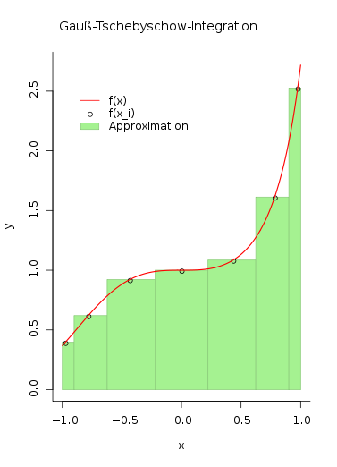
Gauß-Tschebyschow-Integration

Eine Variante der Gauß-Integration auf dem Intervall ${\displaystyle [-1,1]}$ ist jene mit der Gewichtsfunktion ${\displaystyle w(x)={\tfrac {1}{\sqrt {1-x^{2}}}}}$. Die dazugehörigen orthogonalen Polynome sind die Tschebyschow-Polynome, deren Nullstellen und damit auch die Stützpunkte der Quadraturformel direkt in analytischer Form vorliegen:

${\displaystyle x_{i,n}=\cos \left({\frac {2i-1}{2n}}\,\pi \right)}$

während die Gewichte nur von der Anzahl der Stützpunkte abhängen:

${\displaystyle \alpha _{i,n}={\tfrac {\pi }{n}}}$.

Die Erweiterung auf beliebige Intervalle ${\displaystyle [a,b]}$ erfolgt durch eine Variablentransformation (siehe unten). Das gesuchte Integral ${\displaystyle \textstyle \int _{-1}^{1}\,f(x)\,\mathrm {d} x}$ kann umgeformt werden in ${\displaystyle \textstyle \int _{-1}^{1}w(x)\,{\sqrt {1-x^{2}}}\,f(x)\,\mathrm {d} x}$. Zur numerischen Berechnung wird das Integral nun durch die Summe ${\displaystyle \textstyle {\tfrac {\pi }{n}}\,\sum _{i=1}^{n}f(x_{i})\,{\sqrt {1-x_{i}^{2}}}}$ approximiert. Durch Einsetzen der Stützpunkte in analytischer Form erhält man

${\displaystyle \int _{-1}^{1}\,f(x)\,\mathrm {d} x\approx {\tfrac {\pi }{n}}\,\sum _{i=1}^{n}f\left(\cos \left({\tfrac {2i-1}{2n}}\,\pi \right)\right)\,\sin \left({\tfrac {2i-1}{2n}}\,\pi \right)}$,

was der n-fachen Anwendung der Mittelpunktsregel über dem Intervall 0 bis Pi entspricht. Der Fehler kann für einen geeigneten Wert für t zwischen 0 und Pi abgeschätzt werden über

${\displaystyle {\frac {d^{2n}\,\sin \,t\,f(\cos \,t)}{dt^{2n}}}\,\left({\frac {\pi }{2n}}\right)^{2n}\,{\frac {b-a}{(2n+1)!}}.}$

Gauß-Hermite-Integration

Gauß-Integration auf dem Intervall ${\displaystyle (-\infty ,\infty )}$. Es gilt ${\displaystyle w(x)=e^{-x^{2}}}$. Die resultierenden orthogonalen Polynome sind die Hermite-Polynome. Das gesuchte Integral ${\displaystyle \textstyle \int _{-\infty }^{\infty }\,f(x)\,\mathrm {d} x}$ kann umgeformt werden in ${\displaystyle \textstyle \int _{-\infty }^{\infty }w(x)\,e^{x^{2}}\,f(x)\,\mathrm {d} x}$. Zur numerischen Berechnung wird es nun durch die Summe ${\displaystyle \textstyle \sum _{i=1}^{n}f(x_{i})\,e^{x_{i}^{2}}\,\alpha _{i}}$ approximiert.

Stützpunkte und Gewichte der Gauß-Hermite-Integration:

n=1	${\displaystyle x_{i}}$	${\displaystyle \alpha _{i}}$	${\displaystyle \alpha _{i}\,e^{x_{i}^{2}}}$
1	0	${\displaystyle {\sqrt {\pi }}\approx 1{,}7724538509055159}$	1,7724538509055159
n=2	${\displaystyle x_{i}}$	${\displaystyle \alpha _{i}}$	${\displaystyle \alpha _{i}\,e^{x_{i}^{2}}}$
1	${\displaystyle -{\frac {1}{\sqrt {2}}}\approx -0{,}707106781187}$	${\displaystyle {\frac {\sqrt {\pi }}{2}}\approx 0{,}886226925453}$	1,46114118266
2	${\displaystyle {\frac {1}{\sqrt {2}}}\approx 0{,}707106781187}$	${\displaystyle {\frac {\sqrt {\pi }}{2}}\approx 0{,}886226925453}$	1,46114118266
n=3	${\displaystyle x_{i}}$	${\displaystyle \alpha _{i}}$	${\displaystyle \alpha _{i}\,e^{x_{i}^{2}}}$
1	${\displaystyle -{\sqrt {\frac {3}{2}}}\approx -1{,}22474487139}$	${\displaystyle {\frac {\sqrt {\pi }}{6}}\approx 0{,}295408975151}$	1,32393117521
2	0	${\displaystyle {\frac {2{\sqrt {\pi }}}{3}}\approx 1{,}1816359006}$	1,1816359006
3	${\displaystyle {\sqrt {\frac {3}{2}}}\approx 1{,}22474487139}$	${\displaystyle {\frac {\sqrt {\pi }}{6}}\approx 0{,}295408975151}$	1,32393117521
n=4	${\displaystyle x_{i}}$	${\displaystyle \alpha _{i}}$	${\displaystyle \alpha _{i}\,e^{x_{i}^{2}}}$
1	−1,65068012389	0,0813128354472	1,2402258177
2	−0,524647623275	0,804914090006	1,05996448289
3	0,524647623275	0,804914090006	1,05996448289
4	1,65068012389	0,0813128354472	1,2402258177

Gauß-Laguerre-Integration

Gauß-Integration auf dem Intervall ${\displaystyle [0,\infty )}$. Es gilt ${\displaystyle w(x)=e^{-x}}$. Die resultierenden orthogonalen Polynome sind die Laguerre-Polynome. Das gesuchte Integral ${\displaystyle \textstyle \int _{0}^{\infty }\,f(x)\,\mathrm {d} x}$ kann umgeformt werden in ${\displaystyle \textstyle \int _{0}^{\infty }w(x)\,e^{x}\,f(x)\,\mathrm {d} x}$. Zur numerischen Berechnung wird es nun durch die Summe ${\displaystyle \textstyle \sum _{i=1}^{n}f(x_{i})\,e^{x_{i}}\,\alpha _{i}}$ approximiert.

Stützpunkte und Gewichte der Gauß-Laguerre-Integration:

n=1	${\displaystyle x_{i}}$	${\displaystyle \alpha _{i}}$	${\displaystyle \alpha _{i}\,e^{x_{i}}}$
1	1	1	2,7182818284590451
n=2	${\displaystyle x_{i}}$	${\displaystyle \alpha _{i}}$	${\displaystyle \alpha _{i}\,e^{x_{i}}}$
1	${\displaystyle 2-{\sqrt {2}}\approx 0{,}585786437627}$	${\displaystyle {\frac {1}{4}}\left(2+{\sqrt {2}}\right)\approx 0{,}853553390593}$	1,53332603312
2	${\displaystyle 2+{\sqrt {2}}\approx 3{,}41421356237}$	${\displaystyle {\frac {1}{4}}\left(2-{\sqrt {2}}\right)\approx 0{,}146446609407}$	4,45095733505
n=3	${\displaystyle x_{i}}$	${\displaystyle \alpha _{i}}$	${\displaystyle \alpha _{i}\,e^{x_{i}}}$
1	0,415774556783	0,711093009929	1,07769285927
2	2,29428036028	0,278517733569	2,7621429619
3	6,28994508294	0,0103892565016	5,60109462543
n=4	${\displaystyle x_{i}}$	${\displaystyle \alpha _{i}}$	${\displaystyle \alpha _{i}\,e^{x_{i}}}$
1	0,322547689619	0,603154104342	0,832739123838
2	1,74576110116	0,357418692438	2,04810243845
3	4,53662029692	0,038887908515	3,63114630582
4	9,3950709123	0,000539294705561	6,48714508441

Gauß-Lobatto-Integration

Mit dieser nach Rehuel Lobatto benannten Version wird auf dem Intervall ${\displaystyle [-1,1]}$ integriert, wobei zwei der ${\displaystyle n}$ Stützstellen an den Enden des Intervalls liegen. Die Gewichtsfunktion ist ${\displaystyle w(x)=1}$. Polynome ${\displaystyle f}$ bis zum Grad ${\displaystyle 2n-3}$ werden exakt integriert.

${\displaystyle \int _{-1}^{1}f(x)\mathrm {d} x\,\approx \,\sum _{i=1}^{n}\alpha _{i}f(x_{i})}$

Dabei ist ${\displaystyle x_{1}=-1,\,x_{n}=1}$, und ${\displaystyle x_{2}}$ bis ${\displaystyle x_{n-1}}$ sind die Nullstellen der ersten Ableitung des Legendre-Polynoms ${\displaystyle P_{n-1}}$. Die Gewichte sind

${\displaystyle \alpha _{i}={\frac {2}{n(n-1)P_{n-1}^{2}(x_{i})}}}$

Mit ${\displaystyle n=2}$ ergibt sich die Sehnentrapezregel und mit ${\displaystyle n=3}$ die Simpsonregel.

n	Stützstellen ${\displaystyle x_{i}}$	Gewichte ${\displaystyle \alpha _{i}}$
${\displaystyle 2}$	${\displaystyle \pm 1}$	${\displaystyle 1}$
${\displaystyle 3}$	${\displaystyle 0}$	${\displaystyle {\frac {4}{3}}}$
	${\displaystyle \pm 1}$	${\displaystyle {\frac {1}{3}}}$
${\displaystyle 4}$	${\displaystyle \pm {\sqrt {\frac {1}{5}}}}$	${\displaystyle {\frac {5}{6}}}$
	${\displaystyle \pm 1}$	${\displaystyle {\frac {1}{6}}}$
${\displaystyle 5}$	${\displaystyle 0}$	${\displaystyle {\frac {32}{45}}}$
	${\displaystyle \pm {\sqrt {\frac {3}{7}}}}$	${\displaystyle {\frac {49}{90}}}$
	${\displaystyle \pm 1}$	${\displaystyle {\frac {1}{10}}}$
${\displaystyle 6}$	${\displaystyle \pm {\sqrt {{\frac {1}{3}}-{\frac {2{\sqrt {7}}}{21}}}}}$	${\displaystyle {\frac {14+{\sqrt {7}}}{30}}}$
	${\displaystyle \pm {\sqrt {{\frac {1}{3}}+{\frac {2{\sqrt {7}}}{21}}}}}$	${\displaystyle {\frac {14-{\sqrt {7}}}{30}}}$
	${\displaystyle \pm 1}$	${\displaystyle {\frac {1}{15}}}$
${\displaystyle 7}$	${\displaystyle 0}$	${\displaystyle {\frac {256}{525}}}$
	${\displaystyle \pm {\sqrt {{\frac {5}{11}}-{\frac {2}{11}}{\sqrt {\frac {5}{3}}}}}}$	${\displaystyle {\frac {124+7{\sqrt {15}}}{350}}}$
	${\displaystyle \pm {\sqrt {{\frac {5}{11}}+{\frac {2}{11}}{\sqrt {\frac {5}{3}}}}}}$	${\displaystyle {\frac {124-7{\sqrt {15}}}{350}}}$
	${\displaystyle \pm 1}$	${\displaystyle {\frac {1}{21}}}$

Variablentransformation bei der Gauß-Quadratur

Ein Integral über ${\displaystyle [a,b]}$ wird auf ein Integral über ${\displaystyle [-1,1]}$ zurückgeführt, bevor man die Methode der Gauß-Quadratur anwendet. Dieser Übergang kann durch ${\displaystyle x(t):={\frac {1}{b-a}}(2t-a-b)}$ mit ${\displaystyle x(a)=-1}$ und ${\displaystyle x(b)=1}$ sowie ${\displaystyle t(x):=x^{-1}(x)={\frac {b-a}{2}}x+{\frac {a+b}{2}}}$ und Anwendung der Integration durch Substitution mit ${\displaystyle \mathrm {d} t={\frac {b-a}{2}}\mathrm {d} x}$ auf folgende Weise geschehen:

${\displaystyle \int _{a}^{b}f(t)\,\mathrm {d} t={\frac {b-a}{2}}\int _{-1}^{1}f\left({\frac {b-a}{2}}x+{\frac {a+b}{2}}\right)\,\mathrm {d} x\,.}$

Seien nun ${\displaystyle \left(x_{i}\right)_{i},\left({\tilde {x}}_{i}\right)_{i}}$ die Stützstellen und ${\displaystyle \left(\alpha _{i}\right)_{i},\left({\tilde {\alpha }}_{i}\right)_{i}}$ die Gewichte der Gauß-Quadratur über dem Intervall ${\displaystyle [-1,1]}$, bzw. ${\displaystyle [a,b]}$. Deren Zusammenhang ist also durch

${\displaystyle {\tilde {x}}_{i}={\frac {b-a}{2}}x_{i}+{\frac {a+b}{2}}\,,\quad {\tilde {\alpha }}_{i}={\frac {b-a}{2}}\alpha _{i}\,,}$

gegeben.

Adaptives Gauß-Verfahren

Da der Fehler bei der Gauß-Quadratur, wie oben erwähnt, abhängig von der Anzahl der gewählten Stützstellen ist und sich mit einer größeren Anzahl Stützstellen gerade der Nenner erheblich vergrößern kann, legt dies nahe, bessere Näherungen mit größerem ${\displaystyle n}$ zu erhalten. Die Idee ist, zu einer vorhandenen Näherung ${\displaystyle G_{n}}$ eine bessere Näherung, beispielsweise ${\displaystyle G_{2n+1}}$, zu berechnen, um die Differenz zwischen beiden Näherungen zu betrachten. Sofern der geschätzte Fehler ${\displaystyle \varepsilon :=\left|G_{2n+1}-G_{n}\right|}$ eine gewisse absolute Vorgabe ${\displaystyle \varepsilon _{\text{tol}}}$ überschreitet, ist das Intervall aufzuteilen, sodass auf ${\displaystyle \left[a,{\frac {a+b}{2}}\right]}$ und ${\displaystyle \left[{\frac {a+b}{2}},b\right]}$ die ${\displaystyle G_{n}}$-Quadratur erfolgen kann. Jedoch ist die Auswertung einer ${\displaystyle 2n+1}$ Gauß-Quadratur ziemlich kostspielig, da insbesondere für ${\displaystyle n<m}$ im Allgemeinen ${\displaystyle m}$ neue Stützstellen berechnet werden müssen, sodass sich für die Gauß-Quadratur mit Legendre-Polynomen die adaptive Gauß-Kronrod-Quadratur anbietet.

Adaptive Gauß-Kronrod-Quadratur

Die präsentierte Kronrod-Modifikation, welche nur für die Gauß-Legendre-Quadratur existiert, basiert auf der Verwendung der bereits gewählten ${\displaystyle n}$ Stützstellen und der Hinzunahme von ${\displaystyle n+1}$ neuen Stützstellen.^[4] Während die Existenz optimaler Erweiterungen für die Gauß-Formeln von Szegö belegt wurde, leitete Kronrod (1965) für die Gauß-Legendre-Formeln optimale ${\displaystyle n+1}$ Punkte her, die den Präzisionsgrad ${\displaystyle 3n+1}$ sicherstellen.^[4] Wenn die mithilfe der erweiterten Knotenzahl von ${\displaystyle 2n+1}$ berechnete Näherung als ${\displaystyle K_{2n+1}}$ definiert wird, lautet die Fehlerschätzung:

Diese kann dann mit einem ${\displaystyle \varepsilon _{\text{tol}}}$ verglichen werden, um dem Algorithmus ein Abbruchkriterium zu geben. Die ${\displaystyle n+1}$ Kronrod-Knoten und -Gewichte zu den ${\displaystyle n}$ Gauß-Legendre-Knoten und -Gewichten sind für ${\displaystyle n\in \{3,7\}}$ in der folgenden Tabelle festgehalten. Die Gauß-Knoten wurden mit einem (G) markiert.

n=3	${\displaystyle x_{i}}$	${\displaystyle \alpha _{i}}$
1	~0,960491268708020283423507092629080	~0,104656226026467265193823857192073
2	~0,774596669241483377035853079956480 (G)	~0,268488089868333440728569280666710
3	~0,434243749346802558002071502844628	~0,401397414775962222905051818618432
4	0 (G)	~0,450916538658474142345110087045571
5	~-0,434243749346802558002071502844628	~0,401397414775962222905051818618432
6	~-0,774596669241483377035853079956480 (G)	~0,268488089868333440728569280666710
7	~-0,960491268708020283423507092629080	~0,104656226026467265193823857192073
n=7	${\displaystyle x_{i}}$	${\displaystyle \alpha _{i}}$
1	~0,991455371120812639206854697526329	~0,022935322010529224963732008058970
2	~0,949107912342758524526189684047851 (G)	~0,063092092629978553290700663189204
3	~0,864864423359769072789712788640926	~0,104790010322250183839876322541518
4	~0,741531185599394439863864773280788 (G)	~0,140653259715525918745189590510238
5	~0,586087235467691130294144838258730	~0,169004726639267902826583426598550
6	~0,405845151377397166906606412076961 (G)	~0,190350578064785409913256402421014
7	~0,207784955007898467600689403773245	~0,204432940075298892414161999234649
8	0 (G)	~0,209482141084727828012999174891714
9	~-0,207784955007898467600689403773245	~0,204432940075298892414161999234649
10	~-0,405845151377397166906606412076961 (G)	~0,190350578064785409913256402421014
11	~-0,586087235467691130294144838258730	~0,169004726639267902826583426598550
12	~-0,741531185599394439863864773280788 (G)	~0,140653259715525918745189590510238
13	~-0,864864423359769072789712788640926	~0,104790010322250183839876322541518
14	~-0,949107912342758524526189684047851 (G)	~0,063092092629978553290700663189204
15	~-0,991455371120812639206854697526329	~0,022935322010529224963732008058970

Weblinks

• efunda: Abscissas and Weights of Gauss-Laguerre Integration
• WolframMathWorld:Numerische Integration (englisch)

Literatur

• Philip J. Davis, Philip Rabinowitz: Methods of Numerical Integration. 2. Auflage. Academic Press, Orlando FL u. a. 1984, ISBN 0-12-206360-0.
• Vladimir Ivanovich Krylov: Approximate Calculation of Integrals. MacMillan, New York NY u. a. 1962.
• Arthur H. Stroud, Don Secrest: Gaussian Quadrature Formulas. Prentice-Hall, Englewood Cliffs NJ 1966.
• Arthur H. Stroud: Approximate Calculation of Multiple Integrals. Prentice-Hall, Englewood Cliffs NJ 1971, ISBN 0-13-043893-6.
• Martin Hermann: Numerische Mathematik, Band 2: Analytische Probleme. 4., überarbeitete und erweiterte Auflage. Walter de Gruyter Verlag, Berlin und Boston 2020. ISBN 978-3-11-065765-4.

Quellen

1. ↑ Methodus nova integralium valores per approximationem inveniendi. In: Comm. Soc. Sci. Göttingen Math. Band 3, 1815, S. 29–76, Gallica, datiert 1814, auch in Werke, Band 3, 1876, S. 163–196.
2. ↑ C. G. J. Jacobi: Ueber Gauß’ neue Methode, die Werthe der Integrale näherungsweise zu finden. In: Journal für Reine und Angewandte Mathematik. Band 1, 1826, S. 301–308, (online), und Werke, Band 6.
3. ↑ Philip J. Davis: Interpolation and approximation. [1st ed.]. Blaisdell Pub. Co, New York 1963, ISBN 978-0-486-62495-2, S. 344. 
4. ↑ ^{a b} Robert Piessens, Elise de Doncker-Kapenga, Christoph W. Überhuber, David K. Kahaner: QUADPACK: A subrotine package for automatic integration. Springer-Verlag, Berlin/ Heidelberg/ New York 1983, S. 16–17.